Brief overview into how to best use Google Sheets + some tips so it’s effective for you and your team.

Creating Tables (Alternating Colours)

You can create a table which has rows with alternating colours in Format > Alternating Colours after selecting all the cells in your table. This will bring up a few options including whether or not your table has a header / footer. This is useful for improving the readability of your spreadsheet.

Conditional Formatting

You can create conditional formatting which allows you to visualize your data by selecting the cells and using the menu option Format > Conditional Formatting. You can select colours for the cell text and highlight based on the cell contents.

Decimal Places

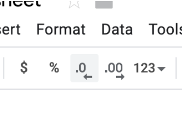
You can change the number of decimal places displayed for a number value in a cell by pressing the increase / decrease decimal places buttons located below the Format and Data menu options.

Formulas

You can apply formulas to cells using the = symbol followed by the formula name such as =UNIQUE. Tooltips will appear showing you what the parameters for the formula are.

Formulas allow you to parse and manipulate data so we can draw key insights from it.

Unique

This formula allows you get all unique values from a selection of cells. So if you want to see what schools people applied from you can use this formula to get a list of all the unique schools.

Sort

If you want to sort some rows (including the list of unique schools) you can use this formula to sort in either ascending or descending order.

Countif

This formula allows you to count the number of instances where a cell in a range matches a criterion cell.

For example if you wanted to count the number of applicants by school you would first use the Unique formula to get all the schools, then you would use the Countif formula to count the instances of each school.

Cell Identities

When applying a formula to multiple cells, any cell references will automatically be shifted in the same direction as the formula; if a cell is applied to a cell below, the cell references will move a cell down.

This is often really useful, especially when multiplying a value in every row by a different value, but there are time when you want to compare a value in every row to a single value or the same set of data (range).

You can select a single cell with the $ symbol on the row and the column: $E$22

To select a single range: $E$22:$F$40

This comes up a lot when comparing one value to a range such as using the Countif formula.

Filters

You can use filters on a table to sort and view data easily, for example if you were looking at applicant data but you only wanted participants’ information you could filter out those that were not accepted.

---

Originally written by Federico Naranjo